Introduction

According to Wolfram Alpha, chaos was defined as the “Irregular unpredictable behavior such as that exhibited by some classes of nonlinear differential equations”. Due to a slight change in initial conditions, a system could exhibit drastically different behaviors. Chaos could be quantified by their Lyanpunov exponent, which was defined as the mean exponential rate of divergence. If a system has a positive Lyanpunov exponent, it implies that the system is chaotic; if a system has only a negative Lyapunov exponent, it implies that the system is non-chaotic.

In this project, we wanted to develop a general method to detect chaos in a system. There are cases where there is a set of deterministic differential equations that governs the system. But very often, in real life, scientist would only obtain a set of data for a system. Examples include in electrical engineering, one may only obtain the voltages across one element in the system, or in economics, one may only obtain one set of values of corn across a time span of five years etc. We would like to have a “canned” method that allows people with either differential equations or experimental data to be able to determine the chaos within the system.

Secondly, we also wanted a method to determine chaos within a generic circuit. An electrical engineer might make a chaotic circuit by mistake. In theory, an inductor would act like a pure inductor and a capacitor would act like a pure capacitor. However, in real life, there are inherent imperfections in an actual inductor and capacitor. An inductor could have capacitive properties, while a capacitor has inductive properties. Moreover, the wires itself also has an inherent resistance and capacitance. Hence, we would like to produce a code that could accept a set of generic data and determine chaos within the circuit.

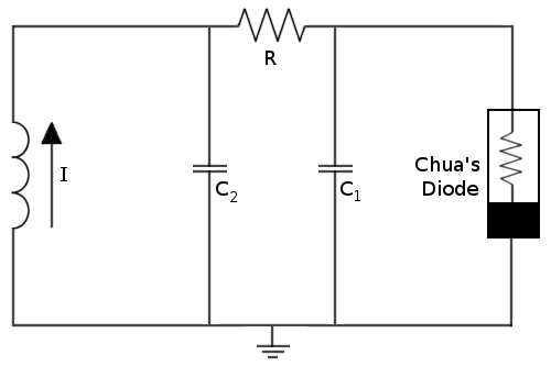
Chua’s circuit [1] is commonly studied circuit. Its popularity comes from the fact that it is easy to construct and that multiple initial conditions could give rise to chaos. In analysis, the voltage going through the capacitors and the current going through the inductor is investigated because capacitors tends to hinder changes in voltage and inductors tend to hinder changes in current.

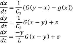
In Chua’s circuit, multiple attractors were discovered [2] and one of the goals of the project was to try to recreate the attractors. The attractor that we focused on in further analysis is the double scroll, because it was a newly found attractor at that time where chaos existed. The differential equations are as follow:

Drawing out Chua's Circuit

RK4 was used to solve the differential equations up to 200,000 time steps. RK4 is one of the most commonly used algorithms to solve differential equations, being both efficient and accurate. A large number of data points were chosen to ensure that there were enough divergences happening in the attractor such that a more accurate average could be taken.

To evaluate whether our algorithms work, we compared different attractors obtained from the analysis of Chua [1] [2]. It was found that the shape of the attractors closely match each other, validating our method of visualizing Chua's Circuit.

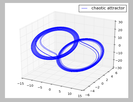
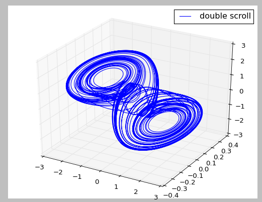
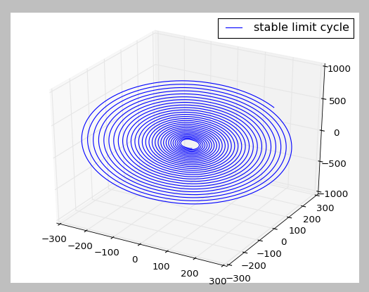
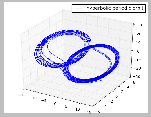
All the pictures are generated from the same differential equations with different initial conditions. The top left picture shows a chaotic attractor with V1 = 9.13959, V2 = -1.35164, I = -59.2869. The top right picture shows a double scroll with V1 = 0.15264, V2 = -0.02281, I = 0.38127. The bottom left picture shows a stable limit cycle with V1 = 1.45305, V2 = -4.36956, I = 0.15034. The bottom right picture shows a hyperbolic periodic orbit with V1 = 10.00717, V2 = 0.80100, I = -23.90375. V1 indicates voltage across capacitor 1, V2 indicates voltage across capacitor 2, I indicates current across inductor.

Determining the Lyapunov Exponent

In Wolf et al. [3], they discussed of a method that determines chaos in an experimental time series. The method includes time-shifting the data sets to obtain three or more sets of data, and then tracking the divergence from a chosen point (called the fiduciary point) on the trajectory constantly. To determine divergence, a near point to the fiduciary point was chosen base on distance and angle from the direction of chaos and was constantly tracked and replaced when the divergence expanded. This method was equivalent to studying an error bar, or two initial conditions with slight differences and tracking their difference in each other as time goes on. As time goes on, the error bar increases exponentially, until the error bar became so large it spans across the 3-space system.

To implement Wolf's method, we first need to determine a "fiduciary point". The fiduciary point would be the point that the program constantly tracks along the trajectory. And to determine how a slight change in initial conditions in the Chua’s circuit would result in drastic differences, the program would need to first evaluate all points on the trajectory and determine the nearest point to the fiduciary point. However, the program also took into consideration that it could not choose nearest points that were immediately before or after the fiduciary point, because the Lyapunov exponent at those points would definitely be zero – the fiduciary point was simply tracing the nearest point. Instead, the program takes a point that is not immediately before or after the fiduciary point but still chose the point closest to the fiduciary point. As the distance between the fiduciary point and the chosen point passes the threshold (which is 2.5% of the total space that the attractor was enclosed in), another “nearest point” was chosen. However, this time, the choice also takes into account the “direction of chaos” – the vector drawn between the candidate point and the fiduciary point needs to be within thirty degrees of the vector drawn between the fiduciary point and the original “nearest point”. This method would then preserve the “direction of chaos”, yielding us a more accurate Lyapunov exponent.

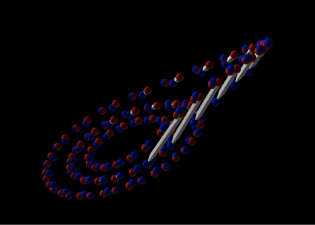
The red point indicates a fiduciary point and the blue point indicates a comparison point. As seen, the points originally started out very close to each other, but the white rods grew increasingly larger. This phenomena is characteristic of chaos and implies that similar initial conditions does not indicate similar final results.

Secondly, we track the divergence from the fiduciary point. The distances between the fiduciary point and the nearest point are monitored until it reaches a threshold, and then the nearest point would be replaced by the aforementioned method.

Lastly, the average exponential growth of distances was calculated. After tracking a series of divergences, we found out that there were “bursts” of growth within the data set. That burst of growth would be determined as the “exponential rate” of divergence. We take the ratio between the final distance and the initial distance between the nearest point and the fiduciary point, and by taking the running average natural log / log base two of the ratio, we could obtain the lyapunov exponent.

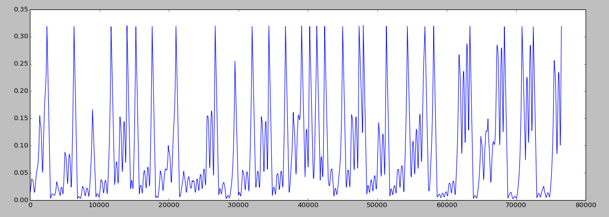
A graph detailing the exponential growth of distances between a fiduciary point and comparison point.

Treating the data Experimentally

In real life, scientists often could only obtain one set of data, which, in this case, would be voltages. Hence, to generate simulated data points, we took only one set of data points (the voltage across the capacitor C1), and time shifted the set by one time delay and two time delays for the voltage across capacitor C2 and current through L respectively. The amount of time delays was repeatedly experimented until we obtain a graph that was relatively similar to the graph with data points solely generated by the three differential equations.

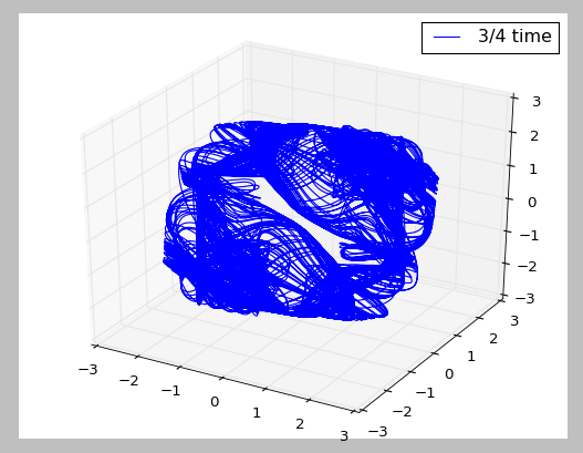
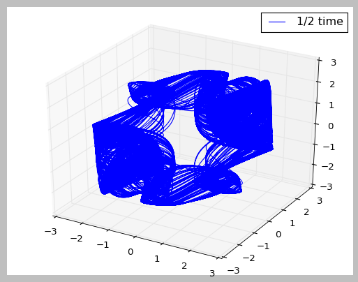
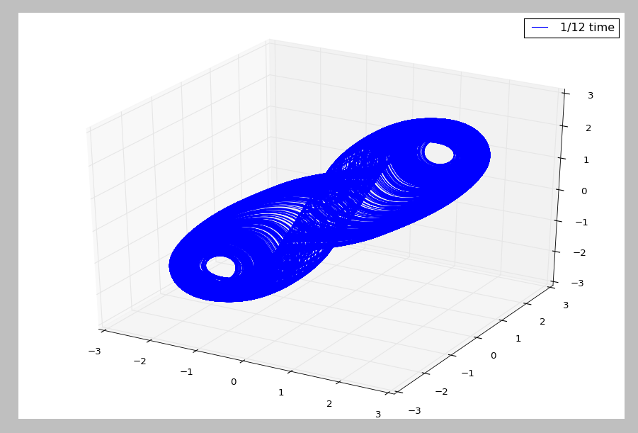
The above graphs shows the “unfolding” of the double scroll of Chua’s circuit. In order, it shows the time shift of a) 3/4, b) 1/2 and c) 1/12 of the mean orbit cycle. The 1/12 mean orbit cycle shows an attractor closest to the double scroll attractor we obtained before, hence validating the time shift and our approach.

Results

The Lyapunov exponent obtained from both value of the differential equations and the simulated experimental data was very close to that of the literature value. From the graph, we also see that the more data points that were taken into consideration, the Lyapunov exponent would converge to the total average, too. Hence, our method was validated through comparison with the literature value and the convergence of the Lyapunov exponent.

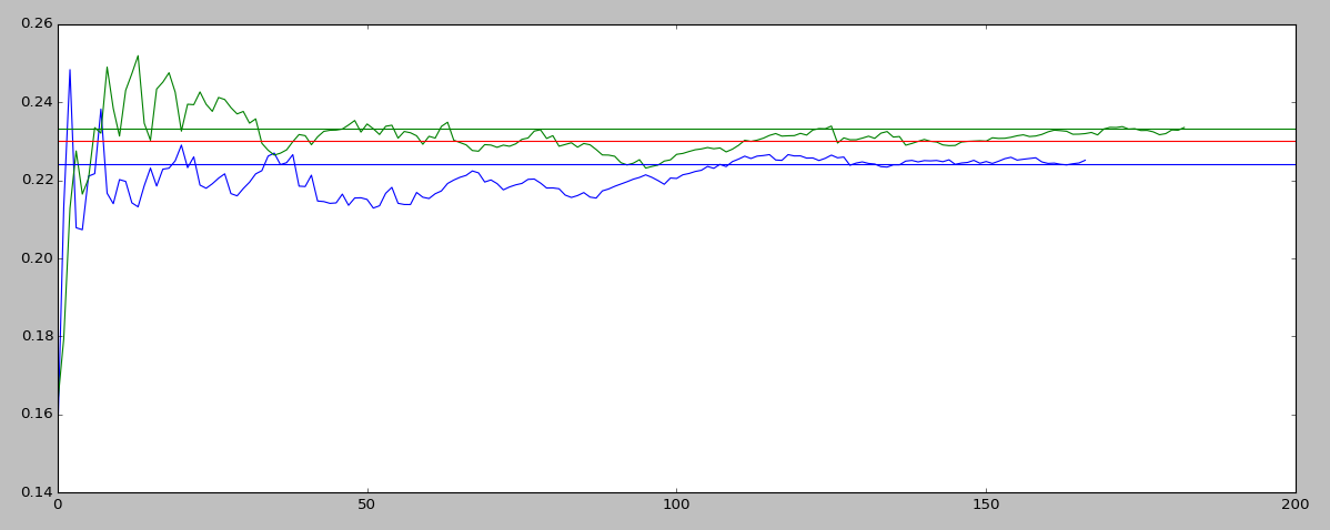
Graph of the running average of the Lyapunov exponent. The y-axis is the Lyapunov exponent while the x-axis is the data points of the obtained lyapunov exponent. The Green lines traces the running average of the lyapunov exponent obtained through data points of the differential equations, while the blue line traces that of simulated experimental data. The red line showed the litereature value, while the green and blue horizontal line showed the total average respectively.

	Literature Value	Value from differential equations	Value from simulated experimental data
Base e	0.23 [2]	0.233	0.226
Base 2	N/A	0.359	0.323

Conclusions and Reflections

The most challenging part of our project was to determine the nearest point the fiduciary point when determining the Lyapunov exponent. We spent a lot of time trying to determine the weighing between a small angle and a small distances, and how to choose if we have candidate points that either aligns perfectly with the direction of chaos but was far away from the fiduciary point or was very near to the fiduciary point but is completely opposite to the direction of chaos. We solved the problem by setting a threshold that the angle between the fiduciary point and a candidate point should be at least 30 degrees apart first. The result turned out well afterwards.

We also have difficulty trying to get the animation to work properly. In Vpython, one frame only supports up to 10,000 lines, hence in our animation, since we have had a lot of data points, the lines started to become “wiggly” at a certain point in time because the program was constantly trying to redraw itself. There was no proper mitigation to this problem, and as the first minute of animation the lines didn’t become too wiggly, we left it as it is in our project.

The easier part of the project was to solve the differential equations and calculating the Lyapunov exponent, since both methods were very standardized and mechanical methods and could be used in a variety of occasions. The generation of graphs was also easy, since it was also a very mechanical process.

In conclusion, apart from the success of the project, we learnt a lot more on quantifying chaos and the multiple methods we could use in computational physics to solve the problem. We also learnt other skills such as problem solving and communication skills between group members.

Reference

[1] Matsumoto, Takashi . "A Chaotic Attractor from Chua's Circuit" (PDF). IEEE Transactions on Circuits and Systems (IEEE). CAS-31 (12): 1055–1058. (1984) Retrieved 2015-11-23.

[2]Matsumoto, T., L. Chua, and M. Komuro. “The Double Scroll.” IEEE Trans. Circuits Syst. IEEE Transactions on Circuits and Systems 32.8 (1985): 797 – 818. Web.

[3]Wolf, Alan. Jack B. Swift, Harry L. Swinney, and John A. Vastano. “Determining the Lyanupov Exponents from a Time Series.” Physica D: Nonlinear Phenomena 16.3 (1985): 285 – 317. Web.

In addition, I would also like to thank my partner Cory Nezin, Professor Alan Wolf for his constant guidance in our project and Professor Anita Raja on giving us guidelines and inspiration for the project.

The code is opensourced. The full code can be found here